In honor of Pi Day : Estimating the value of pi via Monte Carlo simulation

In honor of $\pi$ day, I'll run you through calculating the numerical value of $\pi$ using a method called Monte Carlo simulation. It is basically a type of simulation that samples a lot random values from a distribution. It is used widely to solve many types of problems including those that don't have closed form solutions like estimating the value of numerical integrals, sensitivity analysis, bayesian inference, predicting election results, stock price movements and the list goes on ...

In our scenario, we want to calculate the value of $\pi$. To do this, we''ll be throwing darts at a square dart board (dimensions : 1 by 1) with a quadrant (radius : 1) in it. After throwing a bunch of darts at the board, we'll find the ratio of the number of darts that end up inside the quadrant to the total number of darts we threw and then multiply that number by 4 to get an estimate for the value of $\pi$

Lets work through the math

$4 \times \frac{A_{quadrant}}{A_{square}} = 4 \times \frac{\frac{1}{4}\pi r^{2}}{(1)^2} = 4 \times \frac{\frac{1}{4}\pi(1)^2}{(1)^2} = 4 \times \frac{\frac{1}{4}\pi}{1} \approx  \frac{N_{hits}}{N_{trials}}  \approx   \pi$

In our Monte Carlo simulation, we'll be sampling random points onto our 1 by 1 space and comparing the number of points that end up in the quadrant to the total number of points.

	#!/usr/bin/env python
	# Estimating the value of pi via Monte Carlo simulation
	from random import random
	import sys
	trials = eval(sys.argv[1]) # take input from cli
	hits = 0
	for i in range(trials):
	x, y = random() , random() # generate random x,y in (0,1] at each run
	if x**2 + y**2 < 1 : # defines the edge of the quadrant
	hits = hits + 1
	print 'hits : %d, trials: %d, estimate pi = %1.4F' %(hits, trials, 4*(float(hits) / trials))

view raw pi Monte Carlo v1 hosted with ❤ by GitHub

From the code sample above and my cli, we see that as we increase the number of trials, our estimated value of $\pi$ gets closer to the real value. And if you run enough trials you will approach steady state (true value). Another version of the code sample runs a lot of trials, so you can visually see what's happening to the estimated value of  $\pi$

	#!/usr/bin/env python
	# Estimating the value of pi via Monte Carlo simulation
	from random import random
	import numpy as np
	import matplotlib.pyplot as plt
	trials = list(np.linspace(10,1000000, 1000)) # different number of trials
	pi = []
	def mc_multiple_runs(trials, hits = 0):
	'''
	(float, int) -> (float)
	This function returns the number of hits you get for each monte carlo run
	'''
	for i in range(int(trials)):
	x, y = random() , random() # generate random x,y in (0,1] at each run
	if x**2 + y**2 < 1 : # defines the edge of the quadrant
	hits = hits + 1
	return float(hits)
	for i in trials:
	pi.append(4*(mc_multiple_runs(i)/i))
	print 'hits : %d, trials: %d, estimate pi = %1.4F' %(mc_multiple_runs(i), i, 4*(mc_multiple_runs(i)/i) )
	# plot graphs
	plt.plot(trials, pi, 'g')
	plt.title('Estimating the value of pi via Monte Carlo')
	plt.xlabel('# of Trials')
	plt.ylabel('Estimated value of pi')
	plt.ylim(3.11,3.17)
	plt.show()
	plt.hist(pi, bins = np.linspace(3.12,3.16,50), color='green')
	plt.title('Estimating the value of pi via Monte Carlo')
	plt.xlabel('Estimated value of pi')
	plt.ylabel('Trials')
	plt.xlim(3.13,3.15)
	plt.show()

view raw pi Monte Carlo v2 hosted with ❤ by GitHub

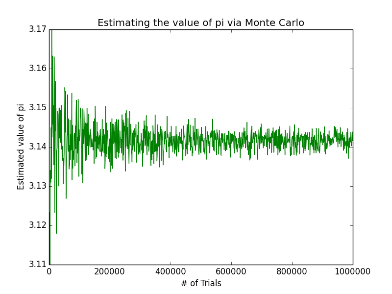
See the graph below. The peaks occur between 3.140 and 3.144, which tells us that the true value of $\pi$ lies somewhere in that range